How OCR Works in Deep Learning: From Text Detection to Sequence Recognition

OCR in context

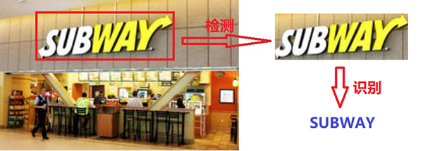
Optical Character Recognition (OCR) is the process of locating text in an image, extracting it, and turning visual character shapes into machine-readable text. At a high level, the system looks for patterns of light and dark, infers character shapes from them, and then maps those shapes to textual symbols.

In practice, OCR is usually divided into two stages:

• Text detection: determine where text appears and define its spatial extent.
• Text recognition: read the detected text region and convert it into character sequences.

Why OCR is difficult

Text detection becomes especially challenging in natural scenes. The main difficulties include:

• text can appear in many different layouts;
• its size and length are highly variable;
• orientation is often not fixed;
• multiple languages may appear in the same image.

How OCR differs from ordinary object detection

Although text detection resembles object detection, the two are not identical:

• Text often forms long rectangles with extreme aspect ratios, unlike many common objects whose width and height are more balanced.
• Ordinary objects such as animals usually have strong closed contours, while text does not.
• A text line consists of multiple characters separated by gaps. If detection is poorly designed, the model may box each character separately instead of capturing the full line.

Typical evaluation criteria

Several practical indicators are commonly used:

• Rejection rate: text that should be recognized is treated as unrecognizable.
• False recognition rate: non-text content is incorrectly recognized as text.
• Recognition speed: acceptable latency is often around 50–500 ms.
• Stability: whether the recognition result stays consistent across similar inputs.

Common applications

OCR is used in a wide range of tasks:

• document and book scanning;
• license plate recognition;
• ID card, card, and receipt recognition;
• educational use cases such as photographing problems for search;
• text recognition pens;
• travel translation apps;
• cameras for visually impaired users;
• automatic navigation systems.

Text detection methods

CTPN (2016)

Core idea

CTPN, short for Detecting Text in Natural Image with Connectionist Text Proposal Network, is one of the influential early deep-learning methods for OCR text detection. Even now, its design still shapes how many OCR detection systems are built.

Its strength lies in detecting horizontal text in natural scenes. Instead of trying to predict a full text line directly, it scans the image with small text proposals of fixed width (16 pixels), identifies local text regions, and then merges those fine-grained proposals into complete text boxes.

Detection process

CTPN proceeds in several steps:

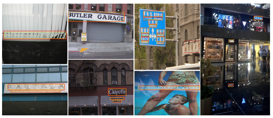
• Local proposal detection: small regions of width 16 pixels are slid across the image. Each proposal uses 10 anchor heights ranging from 11 to 273, scaled by dividing by 0.7 at each step. At every window position, the detector predicts text/non-text scores and vertical coordinates for the anchors.

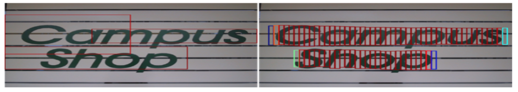
Left: RPN proposals. Right: fine-scale text proposals.

• Proposal connection with RNN: once local text regions are found, they must be linked into meaningful text lines. To reduce false positives from text-like background structures such as windows, bricks, or leaves, CTPN uses a bidirectional LSTM to connect proposals using context from both directions. This recurrent step significantly lowers false detections and also recovers weak text proposals that would otherwise be missed.

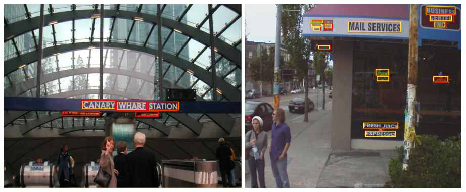
• Side refinement: after linking, the model refines boundaries because the first and last small proposals may not align well with the actual ends of a text line, or edge proposals may be dropped. Text lines are formed by connecting continuous proposals whose text/non-text score is greater than 0.7.

Text-line construction is defined through neighbor pairing. A proposal $B_i$ is considered a paired neighbor of $B_j$ if:

1. it is the nearest in horizontal distance,
2. the horizontal distance is less than 50 pixels,
3. their vertical overlap is greater than 0.7.

If both $B_j \to B_i$ and $B_i \to B_j$ hold, the two proposals are paired, and full text lines are built by sequentially joining such pairs.

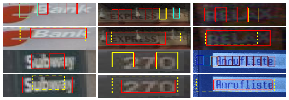
CTPN detection with side refinement (red boxes) and without side refinement (yellow dashed boxes). Colors of the fine-scale proposal boxes indicate text/non-text scores.

Network architecture

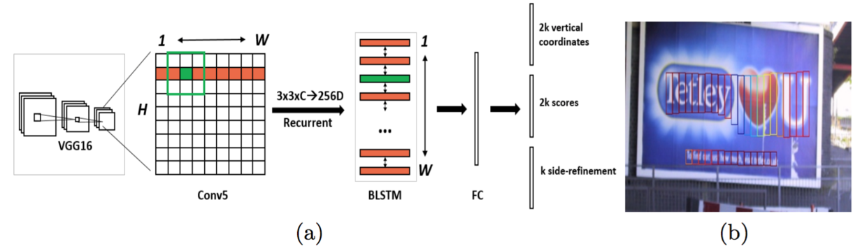
The backbone is VGG16 for feature extraction. On the last convolutional stage, Conv5, a 3×3 convolution is applied to the feature map. While the feature map size depends on the input image, the convolution stride is fixed at 16, and the receptive field is fixed at 228 pixels.

The resulting features are passed to a BLSTM, followed by a fully connected layer that predicts:

• 2K vertical coordinates $y$,
• 2K scores,
• K horizontal offsets for side refinement.

Loss function

CTPN jointly predicts three outputs through the final fully connected layer:

• text/non-text score $s$,
• vertical coordinate regression $v={v_c, v_h}$,
• side-refinement offset $o$.

The loss is:

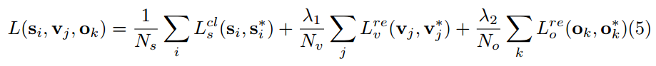
Each anchor is a training sample. Here:

• $s_i$ is the predicted probability that anchor $i$ is text,
• $s_i^*={0,1}$ is the ground truth,
• $v_j$ and $v_j^*$ are predicted and true vertical coordinates,
• $o_k$ and $o_k^*$ are predicted and true x-axis offsets for edge anchors.

Valid anchors for y-coordinate regression are positive anchors or those with IoU > 0.5 against a ground-truth text proposal. Edge anchors are those within a specified horizontal distance from the left or right boundary of a ground-truth text line, for example 32 pixels.

$L_s^{cl}$ is the Softmax classification loss for text vs non-text, and $L_v^{re}$ and $L_o^{re}$ are regression losses. The task weights are set empirically to:

• $\lambda_1 = 1.0$
• $\lambda_2 = 2.0$

$N_s$, $N_v$, and $N_o$ are normalization terms corresponding to the number of anchors used in each loss.

Performance

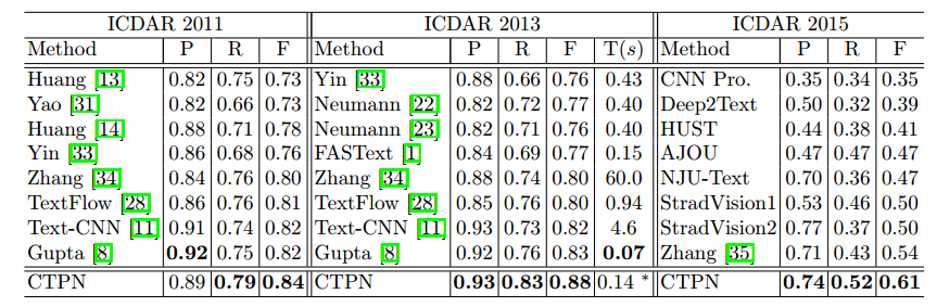
Speed: using a single GPU, complete CTPN detection takes about 0.14 s per image. Removing the RNN connection reduces runtime to about 0.13 s, so the recurrent part adds only a small overhead while delivering a clear accuracy gain.

Accuracy: CTPN performs strongly on scene text detection. On ICDAR 2013, it outperformed methods such as TextFlow and FASText, improving F-measure from 0.80 to 0.88. Precision and recall both increased substantially, by more than +5% and +7% respectively.

It is also relatively good at detecting small text.

The method was evaluated comprehensively on five benchmark datasets.

Weak points

CTPN still has notable limitations:

• It may miss extremely small-scale text.

In very small text regions (inside the red box), some ground-truth boxes are missed. The yellow boxes are ground truth.

• It does not perform well on non-horizontal text.

---

SegLink (2017)

Why orientation matters

General object detectors usually do not need explicit multi-directional handling, but text detection does. Text often has a very large or very small aspect ratio and may appear rotated. If rotated text is still modeled with the usual four parameters $(x, y, w, h)$, localization error can be large. A better fit comes from predicting an additional angle term $\theta$, turning the representation into $(x, y, w, h, \theta)$.

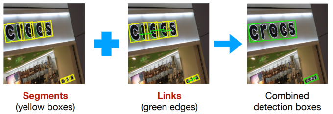
SegLink is a multi-oriented text detector that combines the small-proposal idea of CTPN with the multi-scale detection idea of SSD. Its central insight is to turn text detection into the detection of two local elements:

• segment: an oriented box that covers part of the text;
• link: a connection indicating whether two neighboring segments belong to the same text instance.

By detecting segments and links at multiple scales, the algorithm merges related segments into final text boxes.

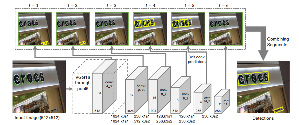
Network structure

The backbone is a pretrained VGG-16 from conv1 to pool5. The original fully connected layers are replaced by convolutional ones:

• fc6 → conv6
• fc7 → conv7

Additional convolution layers from conv8_1 to conv11 are added for multi-scale detection.

The oriented box predicted by the detector is called a segment, denoted as:

$s=(x_s, y_s, w_s, h_s, \theta_s)$

The predictor outputs 7 segment-related channels:

• 2 channels for text/non-text classification,
• 5 channels for geometric regression of the oriented box.

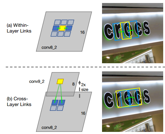
Links between segments

Once segments are detected, they are connected through links:

• Within-layer links: for each segment, the model checks the 8 neighboring segments on the same feature layer to decide whether they belong to the same text.
• Cross-layer links: segments on adjacent feature layers are linked by corresponding index relationships.

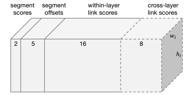
Prediction parameters

For each feature map location, the predictor outputs 31 values in total:

• 2 for segment text/non-text classification;
• 5 for segment geometry $(x, y, w, h, \theta)$;
• 16 for within-layer links: each of 8 directions is a binary classification, so $2 \times 8 = 16$;
• 8 for cross-layer links: 4 links, each binary, so $2 \times 4 = 8$.

So if the current feature map has size $(w, h)$, the output shape is:

$w \times h \times 31$

Merging segments and links

The network produces many segments and links, depending on image size. Before merging, low-confidence predictions are filtered out. Using the retained segments as nodes and retained links as edges, a graph is constructed.

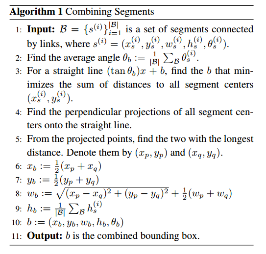
The merging procedure works like this:

• Start with a set $B$ of related segments.
• Each segment has an angle $\theta$; compute the average angle $\theta_b$ over all segments in $B$.
• Fit a line $L$ that minimizes the distances from all segment centers to the line, using least-squares linear regression.
• Project each segment center perpendicularly onto $L$.
• Among all projected points, find the two farthest, denoted $(x_p, y_p)$ and $(x_q, y_q)$.
• The final merged text box is represented as $(x_b, y_b, w_b, h_b, \theta_b)$, where

$$ x_b=\frac{x_p + x_q}{2} \ y_b=\frac{y_q + y_q}{2} $$

• The text-line width $w_b$ is the distance between the two farthest projected points plus half the widths of the segments containing those two points, denoted $W_p$ and $W_q$.
• The text-line height $h_b$ is the average height of all segments.

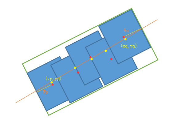
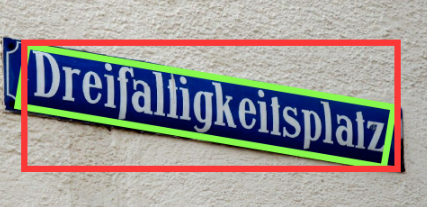
The orange line is the fitted line, red points are segment centers, yellow points are their projections, and the green box is the final merged text box.

Loss function

SegLink uses three losses:

• a Softmax loss for text/non-text classification;
• a Smooth L1 regression loss for box geometry;
• a Softmax loss for link prediction.

The balancing weights $\lambda_1$ and $\lambda_2$ are both set to 1.

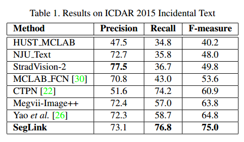
Performance and limitations

For English single-language text detection, SegLink performs better than several competing approaches.

It also handles cluttered backgrounds reasonably well.

In multilingual scenarios, it also shows good accuracy and speed.

Its main shortcomings are:

1. for horizontal text, performance is weaker than CTPN;
2. it struggles with text whose character spacing is very large and with curved text.

Text recognition methods

CRNN + CTC (2015)

While text detection answers where the text is, recognition must answer what the text says. A landmark approach here is CRNN combined with CTC.

Main characteristics

This model has several defining advantages:

1. It is trained end to end, unlike many earlier methods that required separately trained and coordinated components.
2. It naturally handles sequences of arbitrary length without explicit character segmentation or horizontal scale normalization.
3. It is not tied to a predefined vocabulary and works in both lexicon-free and lexicon-based scene text recognition.
4. It yields a compact and efficient model, making it practical for real-world deployment.

Architecture

The network contains three parts:

• a convolutional layer stack to extract a feature sequence from the image;
• a recurrent layer stack to predict a label distribution for each frame;
• a transcription layer to turn frame-wise predictions into the final label sequence.

Feature extraction

The convolutional component is built from a standard CNN without its fully connected layers, using convolution and max-pooling to produce a sequence representation.

Before entering the network, all images are resized to the same height. Feature vectors are then read column by column from left to right from the resulting feature maps. In this setup, each column has width one pixel. The $i$-th feature vector is formed by concatenating the values from the $i$-th column across all feature maps.

Because convolution, max-pooling, and activation operate locally and are translation-invariant, each column in the feature map corresponds to a rectangular region in the original image—its receptive field. So every vector in the extracted sequence can be interpreted as an image descriptor for a local region.

Sequence labeling with recurrent layers

On top of the convolutional features sits a deep bidirectional recurrent neural network. Given the feature sequence $x = x_1, …, x_T$, the recurrent layer predicts a label distribution $y_t$ for each frame $x_t$.

This recurrent stage is valuable for three reasons:

• it captures context within the sequence, which is crucial because image-based symbols are often easier to recognize with neighboring information;
• it allows error signals to flow backward into the convolutional layers, enabling joint training;
• it naturally works with variable-length inputs.

A standard RNN updates its hidden state using the current input and previous state:

$h_t = g(x_t, h_{t-1})$

and predicts $y_t$ from $h_t$. However, vanilla RNNs suffer from the vanishing gradient problem, limiting long-range context modeling.

To address that, CRNN uses LSTM units. An LSTM consists of:

• a memory cell,
• an input gate,
• an output gate,
• a forget gate.

This design allows it to preserve useful context over longer spans and selectively discard irrelevant information. Since image sequences benefit from context in both directions, CRNN uses bidirectional LSTM, combining a forward LSTM and a backward LSTM. Multiple bidirectional LSTM layers can be stacked to form a deep bidirectional LSTM, enabling higher-level sequence abstractions.

Transcription: from frame predictions to text

The transcription stage converts frame-level predictions into a final label sequence. In this setup there are two modes:

• lexicon-free transcription;
• lexicon-based transcription.

The probability model comes from the Connectionist Temporal Classification (CTC) layer. CTC defines the probability of a label sequence $l$ given frame-wise predictions $y = y_1, …, y_T$ without requiring explicit alignment between characters and frames.

Probability of a label sequence

Let each frame prediction be:

$y_t \in \Re^{|{\cal L}'|}$

where ${\cal L}' = {\cal L} \cup$ blank, and the blank label is written as -.

A mapping function ${\cal B}$ transforms a path $\boldsymbol{\pi} \in {\cal L}'^T$ into a label sequence by first removing repeated labels and then deleting blanks. For example:

“–hh-e-l-ll-oo–” maps to “hello”.

The conditional probability is defined as:

$$ \begin{equation} p(\mathbf{l}|\mathbf{y})=\sum_{\boldsymbol{\pi}:{\cal B}(\boldsymbol{\pi})=\mathbf{l}}p(\boldsymbol{\pi}|\mathbf{y}),\tag{1} \end{equation} $$

where

$p(\boldsymbol{\pi}|\mathbf{y})=\prod_{t=1}^{T}y_{\pi_t}^{t}$

and $y_{\pi_t}^{t}$ is the probability of label $\pi_t$ at time $t$.

Because the number of paths grows exponentially, direct summation is infeasible, but the forward algorithm from CTC computes it efficiently.

Lexicon-free transcription

In lexicon-free mode, the predicted label sequence is taken as the one with the highest probability under Equation (1). Exact search is not practical, so an approximation is used:

$$ \mathbf{l}^{*}\approx{\cal B}(\arg\max_{\boldsymbol{\pi}}p(\boldsymbol{\pi}|\mathbf{y})) $$

That is, at each time step, choose the most probable label, then apply ${\cal B}$.

Lexicon-based transcription

In lexicon-based mode, each test sample is associated with a dictionary ${\cal D}$, and prediction becomes:

$$ \mathbf{l}^{*}=\arg\max_{\mathbf{l}\in{\cal D}}p(\mathbf{l}|\mathbf{y}) $$

For large lexicons—such as a 50,000-word Hunspell dictionary—exhaustive search is too expensive. A practical shortcut is to note that the lexicon-free prediction is often close to the true answer in edit distance. So the search is restricted to nearest neighbors ${\cal N}_{\delta}(\mathbf{l}')$, where $\mathbf{l}'$ is the lexicon-free prediction and $\delta$ is the maximum edit distance:

$$ \begin{equation} \mathbf{l}^{*}=\arg\max_{\mathbf{l}\in{\cal N}_{\delta}(\mathbf{l}')}p(\mathbf{l}|\mathbf{y}).\tag{2} \end{equation} $$

Candidate search is accelerated using a BK-tree, a metric tree designed for discrete metric spaces. Its search time complexity is:

$O(\log |{\cal D}|)$

where $|{\cal D}|$ is dictionary size. A BK-tree is built offline for each dictionary, and online lookup returns words within edit distance $\leq \delta$.

Training objective

Let the training set be:

${\cal X}= \lbrace I_i,\mathbf{l}i \rbrace i $

where $I{i}$ is a training image and $\mathbf{l}$ is its ground-truth label sequence. The objective is to minimize the negative log-likelihood of the correct sequence:

$$ \begin{equation} {\cal O}=-\sum_{I_{i},\mathbf{l}{i}\in{\cal X}}\log p(\mathbf{l} \end{equation} $$}|\mathbf{y}_{i}),\tag{3

where $\mathbf{y}{i}$ is the output sequence produced from $I$ by the convolutional and recurrent layers.

This objective is important because it can be computed directly from image–label pairs, without manually annotating the position of every individual character.

Training uses stochastic gradient descent, with gradients computed by backpropagation. Specifically:

• in the transcription layer, errors are propagated using the forward algorithm;
• in the recurrent layer, BPTT is used.

For optimization, ADADELTA is employed to compute learning rates automatically for each dimension. Compared with traditional momentum-based methods, it does not require manual learning-rate tuning, and it was found to converge faster.

Results and practical significance

CRNN achieved strong results on four public benchmarks, including IIIT5k, SVT, IC03, and IC13. Experimental comparisons included different lexicon settings such as 50, 1k, 50k, Full, and None for recognition without a lexicon.

The model was also applied to Optical Music Recognition (OMR), where the task is to read sheet music. In that setting, CRNN outperformed two commercial systems, Capella Scan and PhotoScore. Those systems worked reasonably well on clean data, but their performance dropped sharply on synthetic and real-world images because they relied heavily on accurate binarization to detect staff lines and notes. Under poor lighting, noise, or cluttered backgrounds, binarization often fails.

CRNN is more robust because:

• convolutional features tolerate noise and distortion better;
• recurrent layers exploit contextual relationships inside the score.

A note is not recognized only from itself, but also from nearby notes. For example, comparing vertical positions with surrounding notes can help disambiguate recognition.