This field practice focused on evaluating surface water quality on the Shannan campus of Anhui University of Science and Technology. Under the guidance of the instructor, our group collected nine water samples from the river near the west gate of the campus and measured ammonia nitrogen, BOD5, temperature, and pH. The final condition of the river section was judged using both the single-factor method and the Nemerow pollution index.
What the practice was meant to train
The exercise was not limited to taking a few measurements. It was designed to cover the full workflow of water quality monitoring:
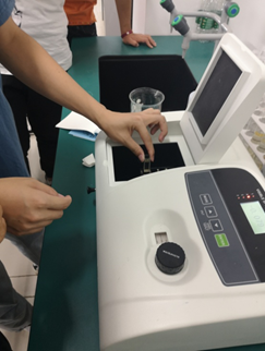
- Independently completing a simulated or real monitoring task, including the use of a spectrophotometer to determine ammonia nitrogen and checking the accuracy and reliability of the operating data.
- Learning how to choose monitoring indicators for a given task, such as DO, temperature, pH, metal content, and BOD, while also selecting suitable sample pretreatment and analytical methods.
- Processing monitoring data scientifically, analyzing each result, making a comprehensive evaluation of water quality, and preparing an assessment report.
- Learning how to divide monitoring sections, arrange sampling points, and collect water samples properly.
Basic sampling principles
Where monitoring sections are typically arranged
For lakes and reservoirs, sampling sections are generally set at:
- inlets and outlets;
- radial lines centered on different functional zones;
- central zones, spawning areas, and retention zones.
In running water systems, monitoring sections can serve different purposes:
- Background section: reflects natural water quality before pollution influence. It should be far from urban residential areas, industrial zones, pesticide and fertilizer application areas, and major traffic corridors.
- Entry section: shows water quality as a watercourse enters an administrative area, before it is affected by local pollution sources.
- Control section: used to show the effect of wastewater discharged from a pollution source or discharge outlet. It should be located downstream where the wastewater and river water are basically mixed.
- Reduction section: used to observe dilution and self-purification downstream of the control section, where major pollutant concentrations have declined significantly.
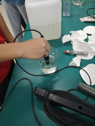
Sampling depth and containers
Samples were taken 0.5 m below the water surface using plastic bottles.
How many verticals and points to use
The number of sampling verticals on a monitoring section depends on the water surface width:
<table> <thead> <tr> <th>Surface width</th> <th>Number of verticals</th> </tr> </thead> <tbody> <tr> <td><=50 m</td> <td>One (center line)</td> </tr> <tr> <td>50~100 m</td> <td>Two (obvious flow zones near left and right banks)</td> </tr> <tr> <td>>100 m</td> <td>Three (left, center, right)</td> </tr> </tbody> </table>Notes:
- Vertical lines should avoid pollution belts; if the pollution belt itself needs to be studied, an additional vertical should be added.
- If the water quality at the section can be shown to be uniform, a single center vertical may be enough.
The number of sampling points on each vertical depends on water depth:
<table> <thead> <tr> <th>Water depth</th> <th>Number of sampling points</th> </tr> </thead> <tbody> <tr> <td><=5 m</td> <td>One upper-layer point</td> </tr> <tr> <td>5~10 m</td> <td>Two points, upper and lower</td> </tr> <tr> <td>>10 m</td> <td>Three points, upper, middle, and lower</td> </tr> </tbody> </table>Further notes:
- The upper layer means 0.5 m below the water surface; if the water is shallower than 0.5 m, sampling is done at half the depth.
- The lower layer means 0.5 m above the riverbed.
- The middle layer is at half the depth.
If pollutant flux needs to be calculated for a section, sampling points must be arranged according to these rules.
Transport and preservation of water samples
Avoiding breakage or loss during transport is basic, but several other points matter just as much:
- Samples should be analyzed as soon as possible after collection, because physical, chemical, and biological changes in the water may affect the results.
- Sample containers should be packed carefully to prevent contamination of the outside, especially around the bottle neck and stopper.
- In winter, samples may freeze; if glass bottles are used, they must be protected from frost cracking.
Common preservation methods include:
- refrigeration or freezing;
- addition of preservation reagents.
Parameters measured in this practice
The work covered pH, dissolved oxygen (DO), ammonia nitrogen, and BOD5.
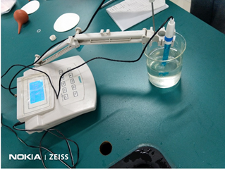
pH measurement
An acidity meter was used, with at least six instruments prepared for the teaching exercise.
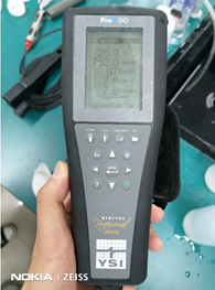
DO measurement
Dissolved oxygen was measured with a DO meter, again with at least six instruments available.
BOD5 measurement
After dilution when necessary, the sample is incubated for five days at 20±1°C. The difference between dissolved oxygen before and after incubation is the BOD5 value. If the five-day biochemical oxygen demand does not exceed 7 mg/L, dilution is not necessary and the sample can be measured directly; many relatively clean rivers fall into this category.
In this practice, DO was measured on the day of sampling and recorded as Day 1. The samples were then incubated in a constant-temperature chamber for five days, after which DO was measured again and recorded as Day 5.
BOD5 = DO (Day 1) - DO (Day 5)
Temperature and pH
Temperature and pH were measured directly at the sampling site on the day of collection.
Determination of ammonia nitrogen by Nessler spectrophotometry
This standard method applies to surface water, groundwater, domestic sewage, and industrial wastewater.
When using a 50 mL sample and a 20 mm cuvette, the method has:
- a detection limit of 0.025 mg/L,
- a lower determination limit of 0.10 mg/L,
- an upper determination limit of 2.0 mg/L,
all expressed as nitrogen.
Principle
In alkaline solution, mercury iodide and potassium iodide react with ammonia to form a light reddish-brown colloidal compound. This product shows strong absorption across a relatively broad wavelength range, and measurement is usually made between 410 and 425 nm.
Ammonia nitrogen present as free ammonia or ammonium ions reacts with Nessler reagent to produce a light reddish-brown complex. The absorbance of this complex is proportional to the ammonia nitrogen concentration, and it is measured at 420 nm.
Interference and how it is handled
A range of organic compounds can interfere, including fatty amines, aromatic amines, aldehydes, acetone, alcohols, and organic chloramines. Inorganic ions such as iron, manganese, magnesium, and sulfur species can also interfere by causing color or turbidity. Natural color and suspended solids in the sample also affect colorimetric measurement.
To remove these effects, pretreatment may include:
- flocculation, sedimentation, and filtration;
- distillation;
- heating under acidic conditions to remove volatile reducing interferents;
- addition of masking agents to suppress metal ion interference.
Specific points noted for this method:
- Suspended matter, residual chlorine, calcium and magnesium ions, sulfides, and organic substances may all interfere.
- If residual chlorine is present, sodium thiosulfate solution can be added to remove it, and starch-potassium iodide paper can be used to check whether chlorine has been fully eliminated.
- During color development, potassium sodium tartrate can reduce interference from calcium, magnesium, and similar metal ions.
- If the water is turbid or colored, predistillation or flocculation-sedimentation pretreatment should be used.
Applicable range
The method has a lowest detectable concentration of 0.025 mol (as stated for the photometric method in the source material) and an upper limit of 2 mg/L. With appropriate pretreatment, it can be applied to surface water, groundwater, industrial wastewater, and domestic sewage.
Instrument
- Spectrophotometer: UV-2800 (UNICO)
Reagents
Water used for reagent preparation must be ammonia-free.
Nessler reagent
Either of the following preparation methods may be used.
Method 1
Dissolve 20 g KI in about 25 mL water. While stirring, add small portions of crystalline HgCl2 powder (about 10 g) until a brick-red precipitate appears and no longer dissolves easily. Then add saturated mercury chloride solution dropwise with continued stirring until a slight brick-red precipitate remains undissolved. Separately dissolve 60 g KOH in water and dilute to 250 mL. After cooling to room temperature, slowly pour the first solution into the KOH solution while stirring, dilute with water to 400 mL, and mix well. Let it stand overnight, then transfer the clear supernatant into a polyethylene bottle and store tightly sealed.
Method 2
Dissolve 16 g NaOH in 50 mL water and cool thoroughly to room temperature. Separately dissolve 7 g KI and 10 g HgI2 in water, then slowly pour this solution into the NaOH solution while stirring. Dilute with water to 100 mL and store in a tightly sealed polyethylene bottle.
Potassium sodium tartrate solution
Dissolve 50 g potassium sodium tartrate (KNaC4H4O6·4H2O) in 100 mL water, boil to remove ammonia, cool, and make up to 100 mL.
Ammonium standard stock solution
Dissolve 3.819 g ammonium chloride (NH4Cl), previously dried at 100°C, in water and dilute to the mark. This solution contains 1.00 mg ammonia nitrogen per mL.
Ammonium standard working solution
Transfer 5.00 mL of the stock solution into a 500 mL volumetric flask and dilute to the mark. This working solution contains 0.010 mg ammonia nitrogen per mL.
Procedure
Calibration curve
Pipette 0, 0.50, 1.00, 4.00, 4.00, 6.00, and 10.0 mL of ammonium standard working solution into 50 mL colorimetric tubes and dilute to the mark with water. Add 1.0 mL potassium sodium tartrate solution and mix. Then add 1.5 mL Nessler reagent and mix again. After standing for 10 min, measure absorbance at 420 nm using a 20 mm cuvette, with water as the reference.
Subtract the absorbance of the zero-concentration blank tube from each reading to obtain corrected absorbance, then plot a calibration curve of ammonia nitrogen content (mg) versus corrected absorbance.
Sample determination
Take an appropriate volume of pretreated sample after flocculation-sedimentation, making sure the ammonia nitrogen content does not exceed 0.1 mg, transfer it to a 50 mL colorimetric tube, dilute to the mark, and add 1.0 mL potassium sodium tartrate solution.
For samples pretreated by distillation, transfer an appropriate volume of distillate into a 50 mL colorimetric tube, add a certain amount of 1 mol/L NaOH to neutralize boric acid, dilute to the mark, and then add 1.5 mL Nessler reagent. Mix well and let stand for 10 min, then measure absorbance as in the calibration step.
For the blank test, use ammonia-free water instead of sample and carry it through the full procedure.
Subtract the absorbance of the blank from the sample absorbance, then read the ammonia nitrogen content from the calibration curve.
Precision and accuracy
For spiked samples containing 1.14~1.16 mg/L ammonia nitrogen analyzed by three laboratories, the relative standard deviation within a single laboratory did not exceed 9.5%, and the recovery ranged from 95% to 104%.
For spiked samples containing 1.81~3.06 mg/L analyzed by four laboratories, the relative standard deviation within a single laboratory did not exceed 4.4%, and the recovery ranged from 94% to 96%.
Notes
- The ratio of mercury iodide to potassium iodide in Nessler reagent has a major influence on the sensitivity of the color reaction. Any precipitate formed after standing should be removed.
- Filter paper often contains trace ammonium salts, so it should be rinsed with ammonia-free water before use. Glassware should also be protected from contamination by ammonia in laboratory air.
Water quality evaluation methods
Two methods were used to assess the sampled river section.
1. Single-factor evaluation
$$ I_i\=\frac{C_i}{S_i} $$
Where:
- $I_i$: environmental quality index of the pollutant;
- $C_i$: measured concentration of the pollutant, $mg/m^3$;
- $S_i$: environmental quality standard for the pollutant.
A smaller $I_i$ value indicates better quality. If $I_i<1$, the indicator meets the standard; if $I_i>1$, it exceeds the standard.
This expresses the degree to which the actual concentration surpasses the evaluation standard.
2. Nemerow pollution index
$$ P\=\sqrt{\frac{I_{imax}^{2}+I_{iave}^{2}}{2}} $$
Where:
- $I_{imax}$: the maximum value among the single-factor environmental quality indices;
- $I_{iave}$: the average value of the single-factor environmental quality indices.
Water quality classification based on the Nemerow index:
<table> <thead> <tr> <th>P</th> <th>Water quality class</th> </tr> </thead> <tbody> <tr> <td><1</td> <td>Clean</td> </tr> <tr> <td>1\~2</td> <td>Slightly polluted</td> </tr> <tr> <td>2\~3</td> <td>Polluted</td> </tr> <tr> <td>3\~5</td> <td>Heavily polluted</td> </tr> <tr> <td>>5</td> <td>Severely polluted</td> </tr> </tbody> </table>Group arrangement for the field practice
Two classes were divided into 12 groups. Each instructor led four groups to collect surface water samples from the AUST Shannan campus. The collected samples were brought back to the laboratory for measurement of pH, DO, ammonia nitrogen, and BOD5.
Measured results from the west-gate river samples
The following table lists the measured ammonia nitrogen concentration, BOD5, and DO for the nine samples, along with the corresponding Class V standard limits and single-factor indices.
<table> <thead> <tr> <th>Ammonia nitrogen (mg/L)</th> <th>Class V limit for ammonia nitrogen</th> <th>Single factor</th> <th>BOD5</th> <th>Class V limit for BOD5</th> <th>Single factor</th> <th>DO</th> <th>Class V limit for DO</th> <th>Single factor</th> </tr> </thead> <tbody> <tr> <td>0.398</td> <td>2</td> <td>0.20</td> <td>0.77</td> <td>10</td> <td>0.08</td> <td>7.10</td> <td>2</td> <td>0.28</td> </tr> <tr> <td>0.5034</td> <td>2</td> <td>0.25</td> <td>0.81</td> <td>10</td> <td>0.08</td> <td>6.80</td> <td>2</td> <td>0.29</td> </tr> <tr> <td>0.4454</td> <td>2</td> <td>0.22</td> <td>0.57</td> <td>10</td> <td>0.06</td> <td>7.00</td> <td>2</td> <td>0.29</td> </tr> <tr> <td>0.3873</td> <td>2</td> <td>0.19</td> <td>3.34</td> <td>10</td> <td>0.33</td> <td>6.70</td> <td>2</td> <td>0.30</td> </tr> <tr> <td>0.5293</td> <td>2</td> <td>0.26</td> <td>2.82</td> <td>10</td> <td>0.28</td> <td>7.30</td> <td>2</td> <td>0.27</td> </tr> <tr> <td>0.4776</td> <td>2</td> <td>0.24</td> <td>2.54</td> <td>10</td> <td>0.25</td> <td>7.40</td> <td>2</td> <td>0.27</td> </tr> <tr> <td>0.5013</td> <td>2</td> <td>0.25</td> <td>1.65</td> <td>10</td> <td>0.17</td> <td>7.40</td> <td>2</td> <td>0.27</td> </tr> <tr> <td>0.5142</td> <td>2</td> <td>0.26</td> <td>2.15</td> <td>10</td> <td>0.22</td> <td>7.40</td> <td>2</td> <td>0.27</td> </tr> <tr> <td>0.5099</td> <td>2</td> <td>0.25</td> <td>1.20</td> <td>10</td> <td>0.12</td> <td>6.50</td> <td>2</td> <td>0.31</td> </tr> <tr> <td>Average</td> <td></td> <td>0.24</td> <td></td> <td></td> <td>0.18</td> <td></td> <td></td> <td>0.28</td> </tr> </tbody> </table>From the single-factor results alone, all three indicators remained well below 1. The average index values were:
- Ammonia nitrogen: 0.24
- BOD5: 0.18
- DO: 0.28
That means every measured parameter met the reference standard used in the calculation.
Among the three, the DO-related index was the largest on average, though it still remained far below the threshold for exceedance. BOD5 gave the lowest average single-factor index, indicating relatively light organic oxygen demand in the sampled water. Ammonia nitrogen also stayed comfortably within the standard limit across all nine samples.
Calibration data for ammonia nitrogen
The calibration data used for spectrophotometric determination were recorded as follows:
<table> <thead> <tr> <th>Ammonia nitrogen content</th> <th>Standard ammonia solution concentration (10 mL final volume)</th> <th>Absorbance</th> </tr> </thead> <tbody> <tr> <td>0</td> <td>0</td> <td>0</td> </tr> <tr> <td>5</td> <td>0.2</td> <td>0.034</td> </tr> <tr> <td>10</td> <td>0.4</td> <td>0.114</td> </tr> <tr> <td>20</td> <td>0.8</td> <td>0.185</td> </tr> <tr> <td>40</td> <td>1.2</td> <td>0.295</td> </tr> <tr> <td>60</td> <td>1.6</td> <td>0.363</td> </tr> </tbody> </table>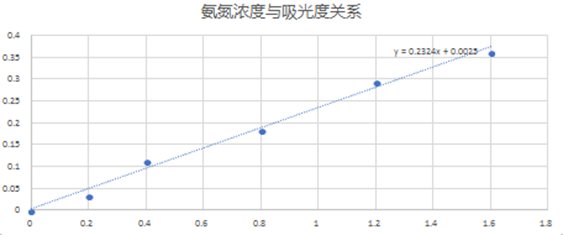
Overall reading of the sampling results
Based on the single-factor assessment, the sampled section of the west-gate river on campus performed well for the measured indicators. The ammonia nitrogen values were all much lower than the Class V limit of 2 mg/L. BOD5 values were also far below the Class V limit of 10 mg/L, with the highest measured value only reaching 3.34 mg/L. Measured dissolved oxygen values ranged from 6.50 to 7.40 mg/L, indicating that the water retained a relatively favorable oxygen condition during sampling.
Using these single-factor indices together with the Nemerow approach provides a more complete picture than any one indicator alone. In this set of samples, none of the measured factors suggested obvious exceedance or severe deterioration in water quality for the river section surveyed.
The practice was valuable not only because it produced a result, but because it connected field layout, sample collection, preservation, instrument operation, data handling, and final evaluation into one continuous monitoring process.